Biased molecular dynamics

The probability density for a geometric parameter ξ of the system driven by a Hamiltonian:

$H(q,p) = T(p) + V(q), \;$

with T(p), and V(q) being kinetic, and potential energies, respectively, can be written as:

$P(\xi_i)=\frac{\int\delta\Big(\xi(q)-\xi_i\Big) \exp\left\{-H(q,p)/k_B\,T\right\} dq\,dp}{\int \exp\left\{-H(q,p)/k_B\,T\right\}dq\,dp} = \langle\delta\Big(\xi(q)-\xi_i\Big)\rangle_{H}.$

The term $\langle X \rangle_H$ stands for a thermal average of quantity X evaluated for the system driven by the Hamiltonian H.

If the system is modified by adding a bias potential $\tilde{V}(\xi)$ acting on one or multiple selected internal coordinates of the system ξ=ξ(q), the Hamiltonian takes a form:

$\tilde{H}(q,p) = H(q,p) + \tilde{V}(\xi),$

and the probability density of ξ in the biased ensemble is:

$\tilde{P}(\xi_i)= \frac{\int \delta\Big(\xi(q)-\xi_i\Big) \exp\left\{-\tilde{H}(q,p)/k_B\,T\right\} dq\,dp}{\int \exp\left\{-\tilde{H}(q,p)/k_B\,T\right\}dq\,dp} = \langle\delta\Big(\xi(q)-\xi_i\Big)\rangle_{\tilde{H}}$

It can be shown that the biased and unbiased averages are related via a simple formula:

$P(\xi_i)=\tilde{P}(\xi_i) \frac{\exp\left\{\tilde{V}(\xi)/k_B\,T\right\}}{\langle \exp\left\{\tilde{V}(\xi)/k_B\,T\right\} \rangle_{\tilde{H}}}.$

More generally, an observable $\langle A \rangle_{H}$:

$\langle A \rangle_{H} = \frac{\int A(q) \exp\left\{-H(q,p)/k_B\,T\right\} dq\,dp}{\int \exp\left\{-H(q,p)/k_B\,T\right\}dq\,dp}$

can be expressed in terms of thermal averages within the biased ensemble:

$\langle A \rangle_{H} =\frac{\langle A(q) \,\exp\left\{\tilde{V}(\xi)/k_B\,T\right\} \rangle_{\tilde{H}}}{\langle \exp\left\{\tilde{V}(\xi)/k_B\,T\right\} \rangle_{\tilde{H}}}.$

Simulation methods such as umbrella sampling use a bias potential to enhance sampling of ξ in regions with low P(ξ_i) such as transition regions of chemical reactions. The correct distributions are recovered afterwards using the equation for $\langle A \rangle_{H}$ above.

A more detailed description of the method can be found in Ref.. Biased molecular dynamics can be used also to introduce soft geometric constraints in which the controlled geometric parameter is not strictly constant, instead it oscillates in a narrow interval of values. The bias potentials are supported both the NVT and NpT MD simulations regardless of the particular thermostat and/or barostat setting. Different types of potentials can be freely combined.

Graphical representation of (a) harmonic, (b) Fermi function-shaped, and (c) and Gauss function-shaped bias potentials.

Supported types of bias potentials

Presently, the following types of bias potential are supported:

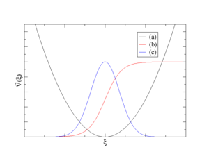
• Harmonic potential (see curve (a) on the plot above)

$\tilde{V}(\xi_1,\dots,\xi_{M}) = \sum_{\mu=1}^{M}\frac{1}{2}\kappa_{\mu} (\xi_{\mu}(q)-\xi_{0,\mu})^2 \;$

where the sum runs all ($M$) coordinates the potential acts upon, which are defined in the ICONST-file by setting the status to 8. The parameters of the potential, $\kappa$ (force constant) and $\xi_0$ (minimum of potential), are defined, respectively, via the keywords SPRING_K and SPRING_R0 in INCAR. Optionally, it is also possible to change the value of $\xi_{0,\mu}$ every MD step at a constant rate defined via parameter SPRING_V. Note that the number of items defined via SPRING_K, SPRING_R0, and SPRING_V must be equal to $M$, otherwise the calculation terminates with an error message. This form of bias potential is employed in several simulation protocols, such as the umbrella sampling, umbrella integration, or steered MD, and is useful also in cases where the $\xi_{\mu}$ values need restrained.

• Fermi function (see curve (b) on the plot above)

$\tilde{V}(\xi_1,\dots,\xi_{M}) = \sum_{\mu=1}^{M}\frac{A_{\mu}}{1+\text{exp}\left [-D_{\mu}\frac{\xi(q)}{\xi_{0,\mu}} -1 \right ]} \;$

where the sum runs all ($M$) coordinates the potential acts upon, which are defined in the ICONST-file by setting the status to 4. The parameters of the potential, $A$ (the height of step), $D$ (controlling the slope around the point $\xi_0$), and $\xi_0$ (position of the step), are defined, respectively, via the keywords

FBIAS_A, FBIAS_D, and FBIAS_R0.  

• Gauss function (see curve (b) on the plot above)

$\tilde{V}(\xi_1,\dots,\xi_{M}) = h\,\sum_{\mu=1}^{M}\text{exp}\left [-\frac{(\xi(q)-\xi_0)^2}{2w^2} \right ], \;$

Andersen thermostat

• For a biased molecular dynamics run with Andersen thermostat, one has to:

1. Set the standard MD-related tags: IBRION=0, TEBEG, POTIM, and NSW
2. Set MDALGO=1 (MDALGO=11 in VASP 5.x), and choose an appropriate setting for ANDERSEN_PROB
3. In order to avoid updating of the bias potential, set HILLS_BIN=NSW
4. Define collective variables in the ICONST-file, and set the STATUS parameter for the collective variables to 5
5. Define the bias potential in the PENALTYPOT-file

Nose-Hoover thermostat

• For a biased molecular dynamics run with Nose-Hoover thermostat, one has to:

1. Set the standard MD-related tags: IBRION=0, TEBEG, POTIM, and NSW
2. Set MDALGO=2 (MDALGO=21 in VASP 5.x), and choose an appropriate setting for SMASS
3. In order to avoid updating of the bias potential, set HILLS_BIN=NSW
4. Define collective variables in the ICONST-file, and set the STATUS parameter for the collective variables to 5
5. Define the bias potential in the PENALTYPOT-file

The values of all collective variables for each MD step are listed in the REPORT-file, check the lines after the string Metadynamics.

---

References

- ↑ a b G. M. Torrie and J. P. Valleau, J. Comp. Phys. 23, 187 (1977).
- ↑ D. Frenkel and B. Smit, Understanding molecular simulations: from algorithms to applications, Academic Press: San Diego, 2002.