Biased molecular dynamics: Difference between revisions
No edit summary |
No edit summary |
||
| Line 58: | Line 58: | ||
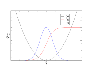
*Fermi function (see curve (b) on the plot above) | *Fermi function (see curve (b) on the plot above) | ||
:<math> | :<math> | ||
\tilde{V}(\xi_1,\dots,\xi_{M}) = \sum_{\mu=1}^{M}\frac{ | \tilde{V}(\xi_1,\dots,\xi_{M}) = \sum_{\mu=1}^{M}\frac{A_{\mu}}{1+\text{exp}\left [-D_{\mu}\frac{\xi(q)}{\xi_{0,\mu}} -1 \right ]} \; | ||
</math> | </math> | ||
where the sum runs all (<math>M</math>) coordinates the potential acts upon, which are defined in the {{FILE|ICONST}}-file by setting the status to 4. | |||
{{TAG|FBIAS_A}} {{TAG|FBIAS_D}} {{TAG|FBIAS_R0}} | |||
*Gauss function (see curve (b) on the plot above) | *Gauss function (see curve (b) on the plot above) | ||
Revision as of 11:57, 6 April 2023
The probability density for a geometric parameter ξ of the system driven by a Hamiltonian:
with T(p), and V(q) being kinetic, and potential energies, respectively, can be written as:
The term stands for a thermal average of quantity X evaluated for the system driven by the Hamiltonian H.
If the system is modified by adding a bias potential acting on one or multiple selected internal coordinates of the system ξ=ξ(q), the Hamiltonian takes a form:
and the probability density of ξ in the biased ensemble is:
It can be shown that the biased and unbiased averages are related via a simple formula:
More generally, an observable :
can be expressed in terms of thermal averages within the biased ensemble:
Simulation methods such as umbrella sampling[1] use a bias potential to enhance sampling of ξ in regions with low P(ξi) such as transition regions of chemical reactions. The correct distributions are recovered afterwards using the equation for above.
A more detailed description of the method can be found in Ref.[2]. Biased molecular dynamics can be used also to introduce soft geometric constraints in which the controlled geometric parameter is not strictly constant, instead it oscillates in a narrow interval of values. The bias potentials are supported both the NVT and NpT MD simulations regardless of the particular thermostat and/or barostat setting. Different types of potentials can be freely combined.

Supported types of bias potentials
Presently, the following types of bias potential are supported:
- Harmonic potential (see curve (a) on the plot above)
where the sum runs all () coordinates the potential acts upon, which are defined in the ICONST-file by setting the status to 8. The parameters of the potential, (force constant) and (minimum of potential), are defined, respectively, via the keywords SPRING_K and SPRING_R0 in INCAR. Optionally, it is also possible to change the value of every MD step at a constant rate defined via parameter SPRING_V. Note that the number of items defined via SPRING_K, SPRING_R0, and SPRING_V must be equal to , otherwise the calculation terminates with an error message. This form of bias potential is employed in several simulation protocols, such as the umbrella sampling[1], umbrella integration, or steered MD, and is useful also in cases where the values need restrained.
- Fermi function (see curve (b) on the plot above)
where the sum runs all () coordinates the potential acts upon, which are defined in the ICONST-file by setting the status to 4.
FBIAS_A FBIAS_D FBIAS_R0
- Gauss function (see curve (b) on the plot above)
Andersen thermostat
- For a biased molecular dynamics run with Andersen thermostat, one has to:
- Set the standard MD-related tags: IBRION=0, TEBEG, POTIM, and NSW
- Set MDALGO=1 (MDALGO=11 in VASP 5.x), and choose an appropriate setting for ANDERSEN_PROB
- In order to avoid updating of the bias potential, set HILLS_BIN=NSW
- Define collective variables in the ICONST-file, and set the STATUS parameter for the collective variables to 5
- Define the bias potential in the PENALTYPOT-file
Nose-Hoover thermostat
- For a biased molecular dynamics run with Nose-Hoover thermostat, one has to:
- Set the standard MD-related tags: IBRION=0, TEBEG, POTIM, and NSW
- Set MDALGO=2 (MDALGO=21 in VASP 5.x), and choose an appropriate setting for SMASS
- In order to avoid updating of the bias potential, set HILLS_BIN=NSW
- Define collective variables in the ICONST-file, and set the STATUS parameter for the collective variables to 5
- Define the bias potential in the PENALTYPOT-file
The values of all collective variables for each MD step are listed in the REPORT-file, check the lines after the string Metadynamics.
References
- ↑ a b G. M. Torrie and J. P. Valleau, J. Comp. Phys. 23, 187 (1977).
- ↑ D. Frenkel and B. Smit, Understanding molecular simulations: from algorithms to applications, Academic Press: San Diego, 2002.
