Liquid Si - Standard MD: Difference between revisions
| (47 intermediate revisions by 2 users not shown) | |||
| Line 131: | Line 131: | ||
*The tag {{TAG|SMASS}} specifies the Nose mass, which is a ficitional mass for the fictional coordinate of the heat bath. The choice of {{TAGBL|SMASS}}=1.0 should work well for this tutorial. | *The tag {{TAG|SMASS}} specifies the Nose mass, which is a ficitional mass for the fictional coordinate of the heat bath. The choice of {{TAGBL|SMASS}}=1.0 should work well for this tutorial. | ||
*Since we are dealing with a super cell, we set {{TAGBL|LREAL}}=Auto. In this mode the projection operators are evaluated in real space. This should speed up the calculation while being slightly less accurate then the evaluation of the operators in reciprocal space. | *Since we are dealing with a super cell, we set {{TAGBL|LREAL}}=Auto. In this mode the projection operators are evaluated in real space. This should speed up the calculation while being slightly less accurate then the evaluation of the operators in reciprocal space. | ||
*To significantly speed up the calculations we use {{TAGBL|ALGO}}=''VeryFast'' and {{TAGBL|PREC}}=''Low''. This is | *To significantly speed up the calculations we use {{TAGBL|ALGO}}=''VeryFast'' and {{TAGBL|PREC}}=''Low''. This is ok for this tutorial example but for more precise results these flags should be used with caution! | ||
*A time step of 3 femtoseconds ({{TAGBL|POTIM}}=3.0) is employed in this example, which should be ok for many applications of Si. | *A time step of 3 femtoseconds ({{TAGBL|POTIM}}=3.0) is employed in this example, which should be ok for many applications of Si. | ||
*The tag {{TAG|NCORE}}=2 specifies that the parallelization is done such that 2 cores share the work on one orbital. This means that for e.g. 8 cores 4 different orbitals would be treated simultaneously, where for each orbital two plane-wave coefficients would be calculated simultaneously. | *The tag {{TAG|NCORE}}=2 specifies that the parallelization is done such that 2 cores share the work on one orbital. This means that for e.g. 8 cores 4 different orbitals would be treated simultaneously, where for each orbital two plane-wave coefficients would be calculated simultaneously. | ||
| Line 140: | Line 140: | ||
It is suggested to run this calculation using the <math>\Gamma</math>-point only version, since we have only one k point. Then it should be a very quick calculation on eight nodes: | It is suggested to run this calculation using the <math>\Gamma</math>-point only version, since we have only one k point. Then it should be a very quick calculation on eight nodes: | ||
mpirun -np 8 vasp_path/vasp_gam | mpirun -np 8 vasp_path/vasp_gam | ||
When the solid melts the crystal structure and the distances between the atoms change. This can be well monitored by looking at the pair correlation function (or radial distribution function). We will also monitor the energy conservation to see if we are well equilibrated. | |||
=== 150 fs === | |||
First we run the calculation for 150 fs. | |||
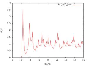
[[File:PC 150fs.jpeg|300px|thumb|Fig. 1: Pair correlation function after 150 fs.]] | |||
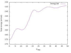
[[File:Energy_150fs.jpg|300px|thumb|Fig. 2: Total energy vs number of steps in first 150 fs.]] | |||
*Pair correlation function: | |||
The pair correlation function is written out to the {{TAG|PCDAT}} file. The abscissa of that file is within mesh points of a selected grid and need to be converted to <math>\AA</math>. This is done by invoking the following short awk script on the command line: | |||
awk <PCDAT >PCDAT.150fs ' NR==8 {pcskal=$1} NR==9 {pcfein=$1} NR>=13 {line=line+1; print (line-0.5)*pcfein/pcskal,$1} ' | |||
This produces the file PCDAT.150fs which contains the pair correlation function against the radius in Angstrom after the first 150 fs (50 timesteps {{TAG|NSW}}=50 with a stepsize of 3 fs {{TAG|POTIM}}=3). | |||
Now we will plot the pair correlation function in the gnuplot window: | |||
gnuplot -e "set xlabel 'r(Ang)'; set ylabel 'PCF'; set style data lines; plot 'PCDAT.150fs'; pause -1" | |||
or to a file (in the remainder we just show how to plot to a file): | |||
gnuplot -e "set terminal jpeg; set xlabel 'r(Ang)'; set ylabel 'PCF'; set style data lines; plot 'PCDAT.150fs'" > PC_150fs.jpg | |||
The obtained pair correlation function should look like in Fig. 1. Solids usually show sharp peaks in the pair correlation function since the ions only vibrate around fixed positions in the crystal lattice. In the liquid or amorphous state the distances are much more diffuse and one usually would expect no far order (but both can have near order). We see that many sharp peaks arise in the pair correlation function at higher distances, so that after 150 fs we have not molten the material. | |||
*Energy conservation: | |||
We will also output the total energy for each molecular dynamics step by invoking the command: | |||
grep "free energy" OUTCAR|awk ' {print $5}' > energy.dat | |||
We will now plot the energy using gnuplot (the user can of course use the plotting program of choice): | |||
gnuplot -e "set terminal jpeg; set xlabel 'N_{step}'; set ylabel 'Total energy (eV/cell)';set style data lines; plot 'energy.dat'" > energy_150fs.jpg | |||
The progression of the total energy with respect to the length of the simulation is shown in Fig. 2. We see that the energy changes very strongly indicating very large changes in the structures. Of course this is related to the melting and it is fine. | |||
=== 300 fs === | |||
We repeat the calculation for another 150 fs. | |||
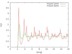
[[File:PC 300fs.jpg|300px|thumb|Fig. 3: Pair correlation functions after 300 and 150 fs.]] | |||
Before we run the calculation we need to copy the new positions and velocities in {{TAG|CONTCAR}} to {{TAG|POSCAR}}. Then rerun the calculation using the same {{TAG|INCAR}} tags and command as above. | |||
*Pair correlation function: | |||
The pair correlation function after 300 fs is written to the file PCDAT.300fs (it is evaluated only in the interval of the last 150 fs since we restarted the calculation): | |||
awk <PCDAT >PCDAT.300fs ' NR==8 {pcskal=$1} NR==9 {pcfein=$1} NR>=13 {line=line+1; print (line-0.5)*pcfein/pcskal,$1} ' | |||
To compare it with the pair correlation function after 150 fs we plot them using the command: | |||
gnuplot -e "set terminal jpeg; set xlabel 'r(Ang)'; set ylabel 'PCF'; set style data lines; plot 'PCDAT.150fs', 'PCDAT.300fs' " > PC_300fs.jpg | |||
The pair correlation functions should look like Fig. 3. We see that after 300 fs much less structure is visible at larger distances. This indicates that the melting is progressing further, but we need to continue with the monitoring of the pair correlation function until it is sufficiently converged. | |||
*Total energy: | |||
We don't look at the total energies here but later. Still the energies from this calculation need to be concatenated to the "energy.dat" file (mind the ">>" instead of ">" above): | |||
grep "free energy" OUTCAR|awk ' {print $5}' >> energy.dat | |||
=== Further continuation === | |||
We continue the calculation for 450 fs. | |||
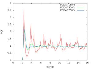
[[File:PC 750fs.jpg|300px|thumb|Fig. 4: Pair correlation functions after 750, 300 and 150 fs.]] | |||
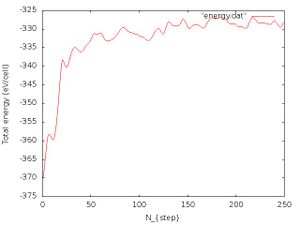
[[File:Energy 750fs.jpg|300px|thumb|Fig. 5: Energy vs number of steps in 750 fs.]] | |||
To do that we first set {{TAG|NSW}}=150 in the {{TAG|INCAR}} file and copy {{TAG|CONTCAR}} to {{TAG|POSCAR}}. | |||
*Pair correlation function: | |||
We obtain the pair correlation function using the command: | |||
awk <PCDAT >PCDAT.750fs ' NR==8 {pcskal=$1} NR==9 {pcfein=$1} NR>=13 {line=line+1; print (line-0.5)*pcfein/pcskal,$1} ' | |||
We compare the pair correlation functions using the command: | |||
gnuplot -e "set terminal jpeg; set xlabel 'r(Ang)'; set ylabel 'PCF'; set style data lines; plot 'PCDAT.150fs', 'PCDAT.300fs', 'PCDAT.750fs' " > PC_750fs.jpg | |||
The pair correlation functions should look like Fig. 4. We see that for 750 fs the peak at 4 <math>\AA</math> got smoothened out compared to 300 fs but the rest of the pair correlation function didn't change much anymore. This is an indication that the calculation is converging. In principle we want to have a well equilibrated structure for a given temperature. | |||
*Total energy: | |||
We will further add the energy data to the ''energy.dat'' file: | |||
grep "free energy" OUTCAR|awk ' {print $5}' >> energy.dat | |||
After that we plot the ''energy.dat'' file: | |||
gnuplot -e "set terminal jpeg; set xlabel 'N_{step}'; set ylabel 'Total energy (eV/cell)';set style data lines; plot 'energy.dat'" > energy_750fs.jpg | |||
The energy vs number of iteration should look like Fig. 5. We see that after a few 100 fs the energy is conserved, but of course with some fluctuations present. This should also indicate that the structure is not changing drastically anymore and that the melting is achieved. We should note that the energy conservation can be monitored because we use the deterministic {{TAG|Nose-Hoover thermostat}} which has a kinetic and potential energy term of the heat bath which provides energy conservation. If we would use e.g. the {{TAG|Langevin thermostat}} which is a stochastic thermostat we would obtain large fluctuations in the total energy. | |||
=== Microcanonical ensemble === | |||
Next we want to continue the calculations but instead of the canonical ensemble ({{TAG|NVT ensemble}}) we are going to carry out the calculations in the microcanonical ensemble ({{TAG|NVE ensemble}}). The microcanonical ensemble calculations are carried out by setting the following tags in the {{TAG|INCAR}} file: | |||
{{TAGBL|MDALGO}} = 1 | |||
{{TAGBL|ANDERSEN_PROB}} = 0.0 | |||
In principle we set here an {{TAG|Andersen thermostat}} but effectively without using it since we set the collision probability of the thermostat {{TAG|ANDERSEN_PROB}} to zero. | |||
We will carry out two hundred more molecular dynamics steps (by setting {{TAG|NSW}}=200) using the microcanonical ensemble. | |||
First we check the mean temperature by typing the following line | |||
grep "mean temperature" OUTCAR | |||
The user should get an output like: | |||
mean temperature <T/S>/<1/S> : 2566.129 | |||
In this example we see that the target temperature is not kept when a microcanonical ensemble is used. | |||
At this point the user should be able to monitor the energies in the calculation. If not repeat from scratch! | |||
'''Exercise:''' Compare the energy conservation of the microcanonical ensemble and the canonical ensemble. Carry out another 200 molecular dynamics steps but with a step size that is only the half of the previous one ({{TAG|POTIM}}=1.5). Compare the energy conservation and check the mean temperature! | |||
=== Further things to try === | |||
To get a better statistics the user should further carry out the calculation for 400-1000 steps in the {{TAG|NVT ensemble}} but with a much smaller time step {{TAGBL|POTIM}}=0.3. '''Repeat the above analysis!''' | |||
== Download == | == Download == | ||
[[Media:Si_Liquid_Melting.tgz| Si_Liquid_Melting.tgz]] | |||
{{Template:Molecular dynamics - Tutorial}} | {{Template:Molecular dynamics - Tutorial}} | ||
[[Category:Examples]] | [[Category:Examples]] | ||
Latest revision as of 09:43, 14 November 2019
Task
Generating liquid Si by melting of the crystalline structure via molecular dynamics.
Input
POSCAR
- We start this example by making a POSCAR using the conventional unit cell with 8 atoms which should look like this:
Si cubic diamond conventional cell
  5.43100000000000
 1.00000000 0.00000000 0.00000000
 0.00000000 1.00000000 0.00000000
 0.00000000 0.00000000 1.00000000
  Si
  8
Direct
  0.00000000 0.00000000 0.00000000
  0.75000000 0.25000000 0.75000000
  0.00000000 0.50000000 0.50000000
  0.75000000 0.75000000 0.25000000
  0.50000000 0.00000000 0.50000000
  0.25000000 0.25000000 0.25000000
  0.50000000 0.50000000 0.00000000
  0.25000000 0.75000000 0.75000000
- We obtain a sufficiently large supercell (2x2x2 containing 64 atoms) by following the description in: Preparing a Super Cell.
- The new POSCAR file of the two 2x2x2 super cell of the conventional cell should look like this:
Si cubic diamond 2x2x2 super cell of conventional cell
     5.43090000000000
    2.00000000   0.00000000   0.00000000
    0.00000000   2.00000000   0.00000000
    0.00000000   0.00000000   2.00000000
   Si
   64
Direct
   0.00000000   0.00000000   0.00000000
   0.50000000   0.00000000   0.00000000
   0.00000000   0.50000000   0.00000000
   0.50000000   0.50000000   0.00000000
   0.00000000   0.00000000   0.50000000
   0.50000000   0.00000000   0.50000000
   0.00000000   0.50000000   0.50000000
   0.50000000   0.50000000   0.50000000
   0.37500000   0.12500000   0.37500000
   0.87500000   0.12500000   0.37500000
   0.37500000   0.62500000   0.37500000
   0.87500000   0.62500000   0.37500000
   0.37500000   0.12500000   0.87500000
   0.87500000   0.12500000   0.87500000
   0.37500000   0.62500000   0.87500000
   0.87500000   0.62500000   0.87500000
   0.00000000   0.25000000   0.25000000
   0.50000000   0.25000000   0.25000000
   0.00000000   0.75000000   0.25000000
   0.50000000   0.75000000   0.25000000
   0.00000000   0.25000000   0.75000000
   0.50000000   0.25000000   0.75000000
   0.00000000   0.75000000   0.75000000
   0.50000000   0.75000000   0.75000000
   0.37500000   0.37500000   0.12500000
   0.87500000   0.37500000   0.12500000
   0.37500000   0.87500000   0.12500000
   0.87500000   0.87500000   0.12500000
   0.37500000   0.37500000   0.62500000
   0.87500000   0.37500000   0.62500000
   0.37500000   0.87500000   0.62500000
   0.87500000   0.87500000   0.62500000
   0.25000000   0.00000000   0.25000000
   0.75000000   0.00000000   0.25000000
   0.25000000   0.50000000   0.25000000
   0.75000000   0.50000000   0.25000000
   0.25000000   0.00000000   0.75000000
   0.75000000   0.00000000   0.75000000
   0.25000000   0.50000000   0.75000000
   0.75000000   0.50000000   0.75000000
   0.12500000   0.12500000   0.12500000
   0.62500000   0.12500000   0.12500000
   0.12500000   0.62500000   0.12500000
   0.62500000   0.62500000   0.12500000
   0.12500000   0.12500000   0.62500000
   0.62500000   0.12500000   0.62500000
   0.12500000   0.62500000   0.62500000
   0.62500000   0.62500000   0.62500000
   0.25000000   0.25000000   0.00000000
   0.75000000   0.25000000   0.00000000
   0.25000000   0.75000000   0.00000000
   0.75000000   0.75000000   0.00000000
   0.25000000   0.25000000   0.50000000
   0.75000000   0.25000000   0.50000000
   0.25000000   0.75000000   0.50000000
   0.75000000   0.75000000   0.50000000
   0.12500000   0.37500000   0.37500000
   0.62500000   0.37500000   0.37500000
   0.12500000   0.87500000   0.37500000
   0.62500000   0.87500000   0.37500000
   0.12500000   0.37500000   0.87500000
   0.62500000   0.37500000   0.87500000
   0.12500000   0.87500000   0.87500000
   0.62500000   0.87500000   0.87500000
KPOINTS
K-Points
 0
Gamma
 1  1  1
 0  0  0
- Since a sufficiently large super cell is used in this example, it is ok in this case to use only a single k-point in the calculations. Hence it is also possible to use the -point only version which is significantly faster than the standard version.
INCAR
ISMEAR = 0
IBRION = 0
MDALGO = 2
ISIF = 2
SMASS = 1.0
SIGMA = 0.1
LREAL = Auto
ALGO = VeryFast
PREC = Low
ISYM = 0
TEBEG = 2000
NSW = 50
POTIM = 3.0
NCORE = 2
- To select a molecular dynamics calculation set IBRION=0.
- By selecting MDALGO=2 and ISIF=2 we select the NVT ensemble using the Nose-Hoover thermostat.
- The tag SMASS specifies the Nose mass, which is a ficitional mass for the fictional coordinate of the heat bath. The choice of SMASS=1.0 should work well for this tutorial.
- Since we are dealing with a super cell, we set LREAL=Auto. In this mode the projection operators are evaluated in real space. This should speed up the calculation while being slightly less accurate then the evaluation of the operators in reciprocal space.
- To significantly speed up the calculations we use ALGO=VeryFast and PREC=Low. This is ok for this tutorial example but for more precise results these flags should be used with caution!
- A time step of 3 femtoseconds (POTIM=3.0) is employed in this example, which should be ok for many applications of Si.
- The tag NCORE=2 specifies that the parallelization is done such that 2 cores share the work on one orbital. This means that for e.g. 8 cores 4 different orbitals would be treated simultaneously, where for each orbital two plane-wave coefficients would be calculated simultaneously.
Calculation
The calculation is started from the perfect crystal. Since the chosen temperature at 2000K is significantly above the known melting temperature at around 1400 K the melting should be achieved relatively quickly.
It is suggested to run this calculation using the -point only version, since we have only one k point. Then it should be a very quick calculation on eight nodes:
mpirun -np 8 vasp_path/vasp_gam
When the solid melts the crystal structure and the distances between the atoms change. This can be well monitored by looking at the pair correlation function (or radial distribution function). We will also monitor the energy conservation to see if we are well equilibrated.
150 fs
First we run the calculation for 150 fs.
- Pair correlation function:
The pair correlation function is written out to the PCDAT file. The abscissa of that file is within mesh points of a selected grid and need to be converted to . This is done by invoking the following short awk script on the command line:
awk <PCDAT >PCDAT.150fs ' NR==8 {pcskal=$1} NR==9 {pcfein=$1} NR>=13 {line=line+1; print (line-0.5)*pcfein/pcskal,$1} '
This produces the file PCDAT.150fs which contains the pair correlation function against the radius in Angstrom after the first 150 fs (50 timesteps NSW=50 with a stepsize of 3 fs POTIM=3). Now we will plot the pair correlation function in the gnuplot window:
gnuplot -e "set xlabel 'r(Ang)'; set ylabel 'PCF'; set style data lines; plot 'PCDAT.150fs'; pause -1"
or to a file (in the remainder we just show how to plot to a file):
gnuplot -e "set terminal jpeg; set xlabel 'r(Ang)'; set ylabel 'PCF'; set style data lines; plot 'PCDAT.150fs'" > PC_150fs.jpg
The obtained pair correlation function should look like in Fig. 1. Solids usually show sharp peaks in the pair correlation function since the ions only vibrate around fixed positions in the crystal lattice. In the liquid or amorphous state the distances are much more diffuse and one usually would expect no far order (but both can have near order). We see that many sharp peaks arise in the pair correlation function at higher distances, so that after 150 fs we have not molten the material.
- Energy conservation:
We will also output the total energy for each molecular dynamics step by invoking the command:
grep "free energy" OUTCAR|awk ' {print $5}' > energy.dat
We will now plot the energy using gnuplot (the user can of course use the plotting program of choice):
gnuplot -e "set terminal jpeg; set xlabel 'N_{step}'; set ylabel 'Total energy (eV/cell)';set style data lines; plot 'energy.dat'" > energy_150fs.jpg
The progression of the total energy with respect to the length of the simulation is shown in Fig. 2. We see that the energy changes very strongly indicating very large changes in the structures. Of course this is related to the melting and it is fine.
300 fs
We repeat the calculation for another 150 fs.
Before we run the calculation we need to copy the new positions and velocities in CONTCAR to POSCAR. Then rerun the calculation using the same INCAR tags and command as above.
- Pair correlation function:
The pair correlation function after 300 fs is written to the file PCDAT.300fs (it is evaluated only in the interval of the last 150 fs since we restarted the calculation):
awk <PCDAT >PCDAT.300fs ' NR==8 {pcskal=$1} NR==9 {pcfein=$1} NR>=13 {line=line+1; print (line-0.5)*pcfein/pcskal,$1} '
To compare it with the pair correlation function after 150 fs we plot them using the command:
gnuplot -e "set terminal jpeg; set xlabel 'r(Ang)'; set ylabel 'PCF'; set style data lines; plot 'PCDAT.150fs', 'PCDAT.300fs' " > PC_300fs.jpg
The pair correlation functions should look like Fig. 3. We see that after 300 fs much less structure is visible at larger distances. This indicates that the melting is progressing further, but we need to continue with the monitoring of the pair correlation function until it is sufficiently converged.
- Total energy:
We don't look at the total energies here but later. Still the energies from this calculation need to be concatenated to the "energy.dat" file (mind the ">>" instead of ">" above):
grep "free energy" OUTCAR|awk ' {print $5}' >> energy.dat
Further continuation
We continue the calculation for 450 fs.
To do that we first set NSW=150 in the INCAR file and copy CONTCAR to POSCAR.
- Pair correlation function:
We obtain the pair correlation function using the command:
awk <PCDAT >PCDAT.750fs ' NR==8 {pcskal=$1} NR==9 {pcfein=$1} NR>=13 {line=line+1; print (line-0.5)*pcfein/pcskal,$1} '
We compare the pair correlation functions using the command:
gnuplot -e "set terminal jpeg; set xlabel 'r(Ang)'; set ylabel 'PCF'; set style data lines; plot 'PCDAT.150fs', 'PCDAT.300fs', 'PCDAT.750fs' " > PC_750fs.jpg
The pair correlation functions should look like Fig. 4. We see that for 750 fs the peak at 4 got smoothened out compared to 300 fs but the rest of the pair correlation function didn't change much anymore. This is an indication that the calculation is converging. In principle we want to have a well equilibrated structure for a given temperature.
- Total energy:
We will further add the energy data to the energy.dat file:
grep "free energy" OUTCAR|awk ' {print $5}' >> energy.dat
After that we plot the energy.dat file:
gnuplot -e "set terminal jpeg; set xlabel 'N_{step}'; set ylabel 'Total energy (eV/cell)';set style data lines; plot 'energy.dat'" > energy_750fs.jpg
The energy vs number of iteration should look like Fig. 5. We see that after a few 100 fs the energy is conserved, but of course with some fluctuations present. This should also indicate that the structure is not changing drastically anymore and that the melting is achieved. We should note that the energy conservation can be monitored because we use the deterministic Nose-Hoover thermostat which has a kinetic and potential energy term of the heat bath which provides energy conservation. If we would use e.g. the Langevin thermostat which is a stochastic thermostat we would obtain large fluctuations in the total energy.
Microcanonical ensemble
Next we want to continue the calculations but instead of the canonical ensemble (NVT ensemble) we are going to carry out the calculations in the microcanonical ensemble (NVE ensemble). The microcanonical ensemble calculations are carried out by setting the following tags in the INCAR file:
MDALGO = 1
ANDERSEN_PROB = 0.0
In principle we set here an Andersen thermostat but effectively without using it since we set the collision probability of the thermostat ANDERSEN_PROB to zero.
We will carry out two hundred more molecular dynamics steps (by setting NSW=200) using the microcanonical ensemble.
First we check the mean temperature by typing the following line
grep "mean temperature" OUTCAR
The user should get an output like:
mean temperature <T/S>/<1/S> : 2566.129
In this example we see that the target temperature is not kept when a microcanonical ensemble is used.
At this point the user should be able to monitor the energies in the calculation. If not repeat from scratch!
Exercise: Compare the energy conservation of the microcanonical ensemble and the canonical ensemble. Carry out another 200 molecular dynamics steps but with a step size that is only the half of the previous one (POTIM=1.5). Compare the energy conservation and check the mean temperature!
Further things to try
To get a better statistics the user should further carry out the calculation for 400-1000 steps in the NVT ensemble but with a much smaller time step POTIM=0.3. Repeat the above analysis!
